
What happened
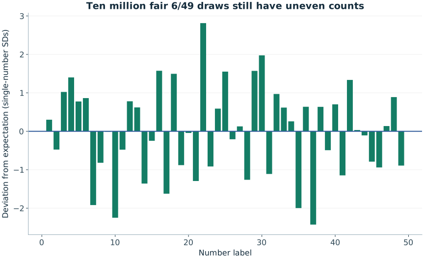
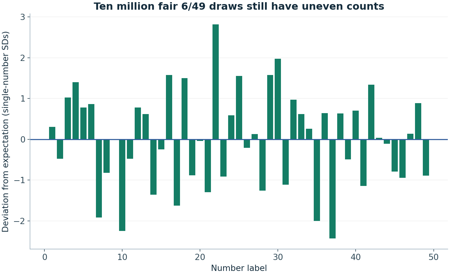
The lowest count was 1,221,974 and the highest was 1,227,407, around a common expectation of 1,224,489.796. At least one adjacent pair appeared in 49.49696% of draws.
The spread is the subject of the experiment, not a ranking to use next time. Every simulated draw used the same label probabilities. The most extreme labels were identified after all 49 counts had been inspected. Their extremeness should not be evaluated as if they had been specified before the run.
Method and benchmark
10,000,000 independent uniform six-number subsets of 1–49. Count every inclusion; compare with N × 6/49. The CSV contains all 49 sufficient frequency totals, not the raw draws.
For a fixed label, X has a binomial marginal distribution with p=6/49 and N=10,000,000. The sum of all counts is exactly 60,000,000. This provides a strong conservation check. The labels’ counts are dependent because each draw contains exactly six selections.
Python 3.12.14 · NumPy 2.3.5 · NumPy PCG64 · seed 20260923. Each experiment starts a separate stream. Code and all datasets are linked below.
What this does not establish
A simulated fair process cannot certify a real lottery. Individual counts are binomial; counts for different numbers are dependent. The maximum is selected after inspecting 49 counts.
The downloadable CSV contains all 49 aggregate counts and their expectations. It does not contain ten million raw lines. The published seed and program regenerate those lines and the reported totals. This compact representation is sufficient to rebuild the frequency figure.
These are original educational simulations prepared for RoomForChance. They are not historical lottery records, a physical-machine audit, an external peer review or evidence of a prediction advantage.
Inspect the data
Download ten-million-649-draws.csv · All results and metadata (JSON) · Download the complete Python program · Download figure-generation code
| number | observed | expected |
|---|---|---|
| 1 | 1,224,802 | 1,224,489.8 |
| 2 | 1,223,997 | 1,224,489.8 |
| 3 | 1,225,551 | 1,224,489.8 |
| 4 | 1,225,943 | 1,224,489.8 |
| 5 | 1,225,294 | 1,224,489.8 |
| 6 | 1,225,385 | 1,224,489.8 |
| 7 | 1,222,500 | 1,224,489.8 |
| 8 | 1,223,641 | 1,224,489.8 |
| 9 | 1,224,478 | 1,224,489.8 |
| 10 | 1,222,159 | 1,224,489.8 |
| 11 | 1,223,994 | 1,224,489.8 |
| 12 | 1,225,299 | 1,224,489.8 |
| 13 | 1,225,134 | 1,224,489.8 |
| 14 | 1,223,080 | 1,224,489.8 |
| 15 | 1,224,234 | 1,224,489.8 |
| 16 | 1,226,122 | 1,224,489.8 |
| 17 | 1,222,807 | 1,224,489.8 |
| 18 | 1,226,040 | 1,224,489.8 |
| 19 | 1,223,577 | 1,224,489.8 |
| 20 | 1,224,445 | 1,224,489.8 |
| 21 | 1,223,149 | 1,224,489.8 |
| 22 | 1,227,407 | 1,224,489.8 |
| 23 | 1,223,541 | 1,224,489.8 |
| 24 | 1,225,101 | 1,224,489.8 |
| 25 | 1,226,099 | 1,224,489.8 |
| 26 | 1,224,275 | 1,224,489.8 |
| 27 | 1,224,622 | 1,224,489.8 |
| 28 | 1,223,182 | 1,224,489.8 |
| 29 | 1,226,119 | 1,224,489.8 |
| 30 | 1,226,538 | 1,224,489.8 |
| 31 | 1,223,339 | 1,224,489.8 |
| 32 | 1,225,496 | 1,224,489.8 |
| 33 | 1,225,129 | 1,224,489.8 |
| 34 | 1,224,758 | 1,224,489.8 |
| 35 | 1,222,419 | 1,224,489.8 |
| 36 | 1,225,151 | 1,224,489.8 |
| 37 | 1,221,974 | 1,224,489.8 |
| 38 | 1,225,149 | 1,224,489.8 |
| 39 | 1,223,980 | 1,224,489.8 |
| 40 | 1,225,217 | 1,224,489.8 |
| 41 | 1,223,301 | 1,224,489.8 |
| 42 | 1,225,875 | 1,224,489.8 |
| 43 | 1,224,524 | 1,224,489.8 |
| 44 | 1,224,379 | 1,224,489.8 |
| 45 | 1,223,671 | 1,224,489.8 |
| 46 | 1,223,515 | 1,224,489.8 |
| 47 | 1,224,631 | 1,224,489.8 |
| 48 | 1,225,412 | 1,224,489.8 |
| 49 | 1,223,565 | 1,224,489.8 |
Reproduce the experiment
Download the Python program to an empty working folder. Use the recorded environment for an exact replay. The program runs all eleven studies and creates a lab-data folder containing the result files. The largest study performs ten million draws; allow time for it to finish.
python -m pip install numpy==2.3.5
python run_experiments.py
Expected CSV SHA-256: 6f7cc9bcd5f49fdfdc25ae10f64180ae8b767b85e365ae7b28678dd21229aba9. A matching seed alone is insufficient if you change the implementation or call sequence. The CSV files use CC BY 4.0; the original code uses the MIT license included with the downloads.
Read the reasoning
Canada LOTTO 6/49: Classic Draw Odds and the Separate Gold Ball Question
Why the Classic Draw has 13,983,816 main combinations and why that denominator does not describe Canada’s separate Gold Ball Draw.
Expected vs Observed Lottery Frequencies: Reading a Table Properly
Learn expected counts, standard deviations and selection effects so a lottery frequency table describes data without pretending to predict the future.
Lottery Number Sums: Why Middle Totals Are Common
Derive the expected sum and variance of a uniform lottery draw, and explain why selecting a common sum does not improve a ticket’s odds.
True Random vs Pseudorandom: Which Difference Matters?
Compare physical entropy and deterministic random streams without confusing reproducibility, statistical quality and cryptographic security.
What Is Randomness? Probability, Patterns and Uncertainty
Understand randomness through fair draws, unpredictable outcomes and the crucial difference between a random process and a random-looking result.
Technical references
NumPy PCG64 documentation describes the generator family. Harvard Stat 110 provides university-level probability background. The model-specific derivation is linked above.