Expected vs Observed Lottery Frequencies: Reading a Table Properly

An observed frequency is a count from a dataset. An expected frequency is the average count predicted by a model over repeated comparable datasets. Their difference is not automatically a defect, a trend or a forecast. Random samples are expected to deviate from their expectations.

A frequency table becomes useful when it shows the sample definition, model, scale of variation and limitations alongside the counts.

Specify the denominator For a fixed label in N independent uniform k-of-n draws, its inclusion probability is p = k/n. The expected count is Np, and its standard deviation is √[Np(1−p)]. The observed proportion is the count divided by N, not by the total number of balls extracted.

If a table instead divides by Nk, it is reporting the share of all extracted labels. That is a different denominator with expectation 1/n. Both can be meaningful, but their percentages must not be compared as if they measured the same quantity.

A worked 6/49 example Over 100 draws, a fixed label has expected count 100×6/49 ≈ 12.245 and standard deviation about 3.278. Over 1,000 draws, the expected count is about 122.449 and standard deviation about 10.366.

The larger sample has a greater typical count deviation but a smaller typical proportional deviation. This is the same absolute-versus-relative distinction illustrated in the law-of-large-numbers experiment.

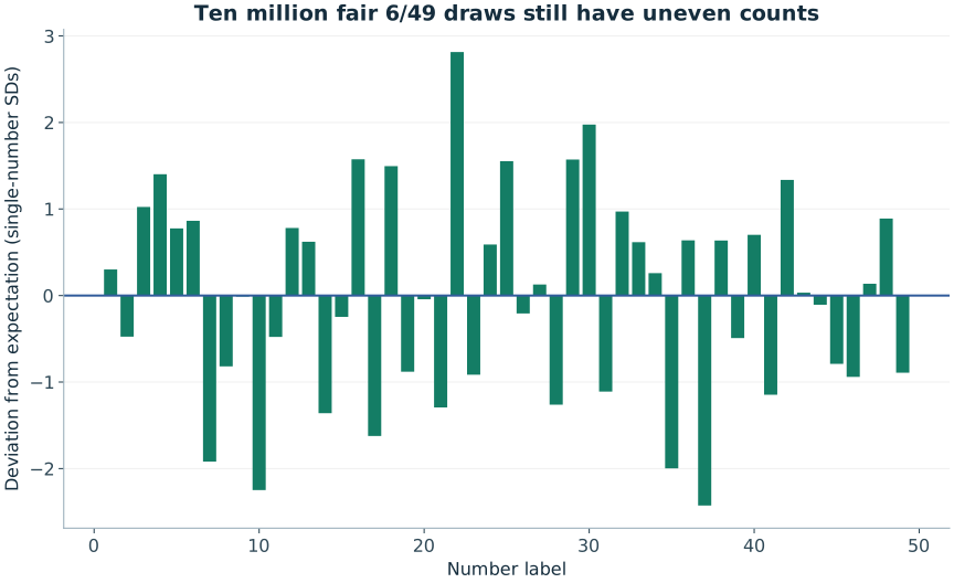
The leader was selected after inspection If you inspect 49 counts and highlight the largest, its extremeness must be judged as the maximum of a collection. A probability statement for one prespecified label does not automatically apply to the label chosen because it looked most unusual.

Moreover, the 49 counts are not independent: every draw contributes exactly six inclusions. Their sum is fixed at 6N. An analysis that models them as 49 independent binomial variables misses that constraint, even though each individual count has a binomial marginal distribution.

What our large simulation contributes Across ten million synthetic 6/49 draws, the smallest label count was 1,221,974 and the largest 1,227,407, with expectation 1,224,489.796 for each label. The figure displays all deviations in units of a fixed label's standard deviation.

That scaling helps compare the counts but is not a simultaneous confidence band and does not turn the selected maximum into a prespecified test. The caption makes that limitation explicit. The CSV includes every count, avoiding selective publication of the most dramatic labels.

Before analysing a historical table Check missing draws, duplicate records, rule changes, different pools and sorted positions. Decide which hypothesis you are testing before choosing a window or statistic. If the question is prediction, reserve genuinely fresh data; a descriptive fit to the table is not enough.

The frequency tool calculates the expectation and spread for one specified label. It does not label observed counts “winning signals”. That restraint is not a missing feature: it is the boundary between describing a sample and claiming knowledge of a future independent draw.