Random Does Not Mean Even: Why Frequencies Fluctuate

If 49 lottery numbers have equal chances, why does a frequency table almost always have a leader and a laggard? Because equal probability describes the process before observations; equal counts would be a very particular result after observations. Fairness produces variation, and sometimes the most suspicious-looking feature of a random sample is its complete absence of variation.

Start with one number, not the whole leaderboard For a specified number in N independent 6/49 draws, each draw is a success with probability p = 6/49. Its count X has mean Np and standard deviation √[Np(1−p)]. At N = 100, the expected count is about 12.24 and the standard deviation is about 3.28. Counts several places apart are therefore unsurprising.

Notice the word specified. We identified the number before inspecting the table. If instead we inspect all 49 numbers and report the largest count, we have selected an extreme. Its distribution is not the same as the count of a number chosen beforehand. Describing the winner of a leaderboard as if it had been predicted is a common statistical mistake.

Larger samples improve proportions, not perfect balance For a fair coin tossed N times, the standard deviation of the number of heads is √N/2. The standard deviation of the proportion of heads is 1/(2√N). As N increases, absolute count differences typically become larger while proportional differences become smaller.

After 100 tosses, being ten heads away from the expected 50 is a ten-percentage-point deviation. After 10,000 tosses, being 100 heads away from the expected 5,000 is only one percentage point. The second sample is further away in count and closer in proportion. These statements are compatible.

Our law-of-large-numbers experiment measures both quantities separately. It also distinguishes mean absolute deviation from standard deviation: both describe spread, but they are not interchangeable statistics.

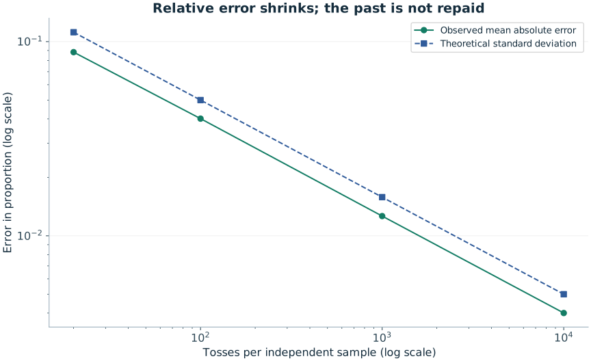
The missing compensation mechanism Suppose a fair coin has produced 60 heads in its first 100 tosses. Its expected number of heads in the next 100 is still 50, not 40. The expected cumulative proportion after the next block is 110/200 = 55%. The proportion moves toward one half because the earlier imbalance is diluted by additional typical observations, not because tails acquire a temporary advantage.

This distinction explains why an apparently reasonable “balancing” strategy becomes the gambler's fallacy. Long-run convergence does not require the future to repay the past.

What a frequency table can legitimately tell you It can describe a sample, help check data quality, and contribute to a properly designed investigation of a mechanism. It cannot turn the most frequent label into a forecast merely by colouring its row red. Before interpreting differences, ask how many draws were included, whether the rules changed, whether the numbers were selected after looking, and how much variation the stated model predicts.

Ten million simulated draws still produce different counts. The Lab publishes all 49 totals so the reader can inspect the complete distribution rather than a sensational headline about the most common number. Equal probabilities survive unequal observations; understanding that distinction is the first step toward reading random data honestly.